
The Hurst Exponent: Reading Persistence in a Price Series

The Hurst exponent turns a price series into a single number between 0 and 1, and the number is usually explained the same way everywhere: above 0.5 the series persists, below 0.5 it reverts, at 0.5 it wanders. That summary is repeated across every tutorial on the subject, and it leaves out the part that decides whether the number means anything.
The reading is not a fixed property of the market. It is the output of an estimator, and it moves with two choices the analyst makes before any market is involved: how far apart the points being compared are, and how much history is fed in. This page shows how far it moves, using series built to have a known answer.
Key takeaways
- The exponent describes how the typical distance travelled grows as the window widens. It is a property of a whole sample, not a statement about the current move.
- On a series built here to have a persistence of 0.7, the same estimator returned 0.798 at a maximum lag of 20 and 0.636 at a maximum lag of 1000. Nothing about the series changed between those two numbers.
- On a series built to be strongly mean-reverting at 0.3, no lag setting tested produced a reading below 0.381. A number near 0.4 does not mean nearly random.
- Sample length matters more than the tutorials suggest. Twenty independent samples of the same 0.7 process, each 250 points long, produced readings from 0.501 to 0.790.
- Every figure on this page is our own computation on synthetic data, run so the true answer is known in advance. No market reading is quoted, because a market reading has no known answer to check it against.
Table of contents
- What the Number Measures, and Over What Window
- The Reading Changes With the Lag You Choose
- Persistence Is Not a Trend You Can Trade Today
- What It Takes to Get a Reading Worth Reading on FX Data
- Price, Log Price or Returns: Three Series, Three Answers
- Where This Fits Before a Strategy Choice, and Where It Does Not
- Who This Page Is Not For
- Frequently Asked Questions
What the Number Measures, and Over What Window
Take a series and ask a simple question: if you compare points two bars apart, how big is the typical gap, and how does that typical gap grow when you compare points twenty bars apart instead? For a series with no memory, the typical distance grows with the square root of the window. The exponent is the power in that relationship, and the square-root case puts it at 0.5.
Above 0.5 the distance grows faster than the square root, which means moves have tended to be followed by moves in the same direction over the sample measured. Below 0.5 it grows more slowly, which means moves have tended to be followed by moves back.
Two things in that description carry the weight. The first is over the sample measured, because the number is one figure summarising the whole history fed in. The second is tended, because the relationship is an average across thousands of comparisons and says nothing about any particular one.
A method built on that distinction rather than on a live signal is closer to what the number can support, and the difference between rule-driven and judgement-driven approaches is set out in the page on systematic and discretionary methods.
The Reading Changes With the Lag You Choose
Every implementation asks for a maximum lag: the widest gap between points that the calculation will consider. Tutorials tend to fill it in with a default and move on. It is not a detail, and the easiest way to show that is to build a series whose answer is already known.
The table below was produced in preparing this page. Two series were generated, one with a built-in persistence of 0.7 and one with a built-in mean reversion of 0.3, then the same estimator was run over each at five maximum-lag settings.
| Maximum lag | Series built at 0.7 | Series built at 0.3 |
|---|---|---|
| 20 | 0.798 | 0.392 |
| 100 | 0.760 | 0.441 |
| 300 | 0.687 | 0.445 |
| 500 | 0.659 | 0.420 |
| 1000 | 0.636 | 0.381 |
The persistent series drifts from 0.798 down to 0.636 as the window widens. A reader handed the first figure would call it strongly trending; handed the last, moderately so. Both came from the same data and the same code.
The mean-reverting column is the more useful half. It was built at 0.3, and the estimator never went below 0.381. Every reading it produced sat closer to 0.5 than to the truth, which means a value around 0.42 on real data is entirely consistent with a strongly mean-reverting series rather than a nearly random one.
So the practical rule is not a recommended lag. It is that a single number carries no information unless the setting that produced it travels with it, and that comparing two readings taken at different settings compares nothing.
Persistence Is Not a Trend You Can Trade Today
A reading above 0.5 says that across the sample, moves have more often been followed by moves the same way than a memoryless series would produce. It does not say the market is trending now, and it does not say the next bar is more likely up than down.
The gap between those two statements is where the measure gets misused. A statistic computed over four thousand bars describes the average behaviour of four thousand bars. Inside that sample there will have been long stretches behaving the opposite way, and the average conceals every one of them.
There is also no direction in the number at all. Persistence is symmetrical: a series that trends hard downward and one that trends hard upward produce the same reading. Anyone treating a high value as bullish has read something into it that is not there.
What it can support is a prior about which family of method has historically suited the instrument, which is a different job from timing. How that prior is then tested rather than assumed is the subject of the page on testing a strategy on history.
What It Takes to Get a Reading Worth Reading on FX Data
The question every tutorial leaves out is how much history the number needs before it stops being noise. It can be answered directly by generating many independent samples of the same process and watching how widely the readings scatter.
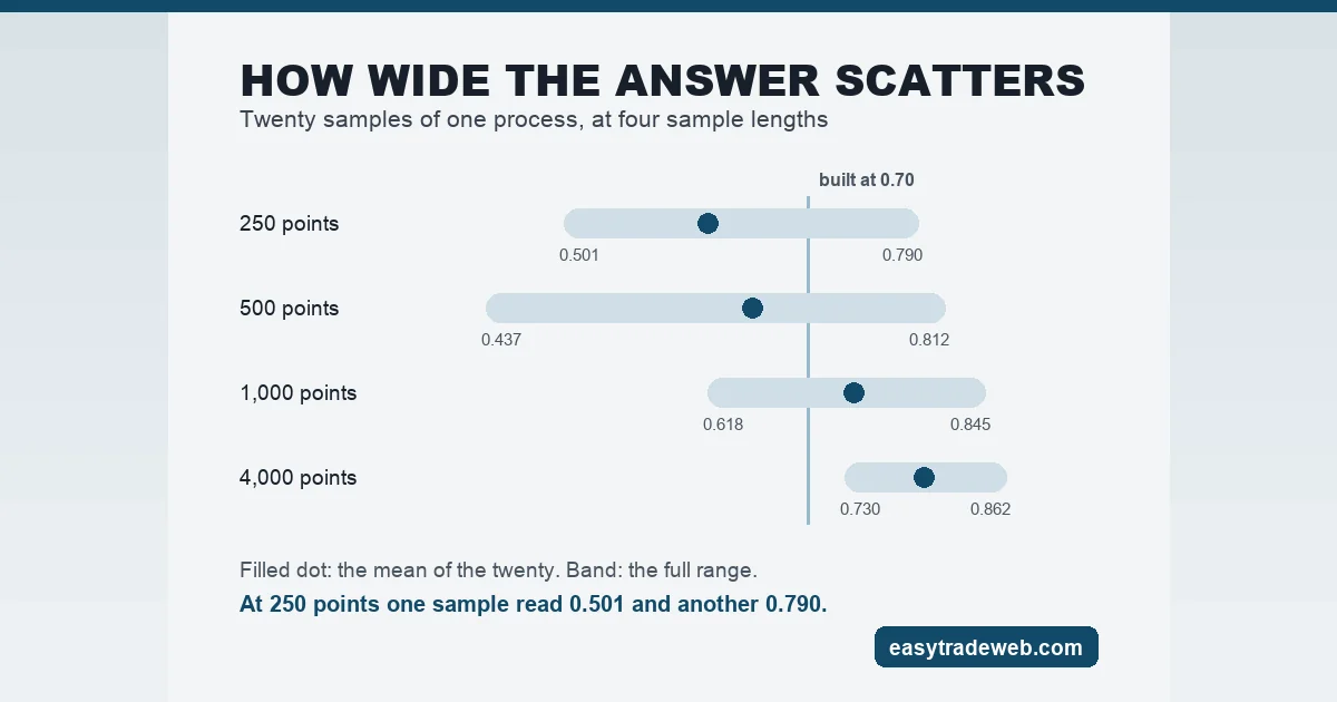
Twenty independent samples were generated at each length below, every one built with the same persistence of 0.7, and the estimator was run over each at a maximum lag of 100.
| Sample length | Mean reading | Range across 20 samples |
|---|---|---|
| 250 points | 0.619 | 0.501 to 0.790 |
| 500 points | 0.655 | 0.437 to 0.812 |
| 1,000 points | 0.738 | 0.618 to 0.845 |
| 4,000 points | 0.795 | 0.730 to 0.862 |
Two hundred and fifty points is roughly a year of daily bars. At that length one sample read 0.501 and another read 0.790, and both were drawn from the identical process. A trader running the calculation once on a year of daily data could have landed anywhere in that range and would have had no way to know it.
At five hundred points the range is wider still, running from 0.437 to 0.812, which includes readings on both sides of 0.5 for a series that is persistent by construction. The scatter only narrows meaningfully by four thousand points.
One further caution belongs with these figures. The mean reading never matched the 0.7 the series was built with at any length tested, and the size and direction of the gap changed as the sample grew. This estimator is not a neutral window onto the underlying property, and treating a single output as that property is the error the whole table is meant to prevent.
Price, Log Price or Returns: Three Series, Three Answers
None of the widely read explanations of this measure is about currencies, and the one decision an FX trader has to make first is which series to run it over. The choice is not cosmetic, because the three candidates are different objects.
The calculation described above operates on a cumulative path, where each value carries the whole history that came before it. A price series is such a path. A returns series is not: it is the set of steps, and running a path estimator over the steps answers a question about the steps rather than about the path.
Log prices sit closer to the assumption the mathematics is built on, because the steps between them are additive and their size does not scale with the level. On an instrument that has spent a long sample far from where it started, the difference between price and log price is not small.
This page states no figure for how much the three differ on a currency pair, because that comparison was not run here and a number produced elsewhere is not evidence. The point that does hold without measurement is that a reading is only comparable with another reading taken over the same construction.
Where This Fits Before a Strategy Choice, and Where It Does Not
The measure is a narrowing device. It can suggest that an instrument has historically rewarded methods that stay with a move rather than fade it, or the reverse, and that suggestion is worth having before committing effort to building one.
It cannot rank two strategies, size a position, or tell anyone when to act. Those decisions come from testing and from risk rules, not from a summary statistic, and a page on trend following as a method covers what actually carries such an approach.
Used honestly, the sequence is short. Compute it at more than one lag setting and on enough history, note the range rather than a single value, and treat the result as a prior about method family that testing may overturn. Used as a signal generator, it produces a number that changes when you change a parameter and rewards whoever tunes it hardest.
The same discipline applies to the loss side of any method the reading points toward, and the way a long adverse run is measured is covered in the page on measuring drawdown.
Who This Page Is Not For
This page does not supply code, a recommended lag, or a threshold at which a market should be traded one way rather than another. It names no instrument as trending or reverting.
It is also not a claim that the measure is useless. It is a demonstration that the output moves with the settings and the sample, and that anyone quoting a single value without both has not yet said anything checkable.
Frequently Asked Questions
What does the Hurst exponent actually measure?
It measures how the typical distance between two points in a series grows as the gap between them widens. A series with no memory grows with the square root of that gap, which corresponds to a value of 0.5. Faster growth gives a higher value and slower growth a lower one, and the figure summarises the whole sample rather than any part of it.
What does a Hurst reading below 0.5 mean?
It means that across the sample measured, moves were more often followed by moves back than a memoryless series would produce. It carries no direction and no timing. The demonstration on this page also shows the reading pulled toward 0.5: a series built at 0.3 never read below 0.381 at any setting tested, so a value near 0.42 can come from a strongly reverting series.
Why does the Hurst exponent change when the lag changes?
Because the maximum lag decides which comparisons enter the calculation. A narrow setting weighs short gaps and a wide one brings in long gaps, and the growth relationship is rarely identical across both. On the series built here at 0.7, the reading fell from 0.798 to 0.636 as the maximum lag went from 20 to 1000 with the data unchanged.
Can the Hurst exponent tell you when to enter a trade?
No. It is a summary of a whole sample and says nothing about the current bar or the next one, and it carries no direction, so the same value can come from a series that rose throughout or one that fell throughout. Treating it as an entry signal asks a sample statistic to answer a question about a single moment.
How much data do you need for a reliable reading?
More than most examples use. Twenty independent samples of one persistent process, each 250 points long, gave readings from 0.501 to 0.790 here, and at 500 points the spread was wider still. The scatter narrowed usefully only at 4,000 points, so a reading taken on a year of daily bars should be treated as one draw from a wide range.
Risk warning: this page is educational and explains what a statistical measure does and does not describe. It is not advice to buy or sell any instrument, it makes no recommendation about any broker, platform or method, and nothing here is a signal or a prediction. Leveraged trading carries a high risk of losing money.